Towards Recommender Engineering
Tools and Experiments for Identifying Recommender Differences
Michael Ekstrand
July 8, 2014
Dedication
This thesis dedicated in memory of John T. Riedl.
Recommender engineering is
- designing and building a recommender system
- for a particular application
- from well-understood principles of algorithm behavior, application needs, and domain properties.
Understand recommendation well enough to build recommenders from requirements.
#1tweetresearch
Different recommender algorithms have different behaviors. I try to figure out what those are.
… in relation to user needs
… so we can design effective recommenders
… because I'm curious
Contributions
Publications
LensKit (RecSys 2011)
CF Survey (Foundations and Trends in HCI)
When Recommenders Fail (RecSys 2012, short)
User study (RecSys 2014)
Grapht (in preparation)
Parameter tuning (in preparation)
Collaborators
- John Riedl
- Joseph Konstan
- Michael Ludwig
- Jack Kolb
- Max Harper
- Lingfei He
- Martijn Willemsen (TU Eindhoven)
Overview
Overview
Recommender Systems

Recommender Systems

recommending items to users
Recommender Approaches
Many algorithms:
- Content-based filtering
- Neighbor-based collaborative filtering [Resnick et al., 1994; Sarwar et al., 2001]
- Matrix factorization [Deerwester et al., 1990; Sarwar et al., 2000; Chen et al., 2012]
- Neural networks [Jennings & Higuchi, 1993; Salakhutidinov et al., 2007]
- Graph search [Aggarwal et al., 1999; McNee et al., 2002]
- Hybrids [Burke, 2002]
Common R&D Practice
- Develop recommender tech (algorithm, UI, etc.)
- Test on particular data/use case
- See if it is better than baseline
- Publish or deploy
Evaluating Recommenders
Many measurements:
- ML/IR-style data set experiments [Herlocker et al., 2004; Gunawardana & Shani, 2009]
- User studies [McNee et al., 2006; Pu et al., 2011; Knijnenburg et al., 2012]
A/B testing [Kohavi]
- Engagement metrics
- Business metrics
Common R&D Practice
- Develop recommender tech (algorithm, UI, etc.)
- Test on particular data/use case
- See if it is better than baseline
- Publish or deploy
Learned: is new tech better for target application?
Not learned: for what applications is new tech better? why?
Algorithms are Different
- Algorithms perform differently
- No reason to believe one size fits all
- Quantitatively similar algorithms can have qualitatively different results [McNee, 2006]
- Different algorithms make different errors
- Opportunity to tailor system to task
- Doesn't even count other system differences!
Human-Recommender Interaction [McNee 2006]
Harness recommender personality to meet specific user information needs
Task-centered design approach
- Interaction
- Algorithm
- Task
Not yet reality!
Requirements for Engineering
To enable recommender engineering, we to understand:
- Algorithm behaviors and characteristics
- Relevant properties of domains, use cases, etc. (applications)
- How these interactions affect suitability
All this needs to be reproduced, validated, and generalizable.
Prior Work
- Diversity [Ziegler et al., 2005; Vargas & Castells, 2011; Bollen et al., 2010]
- Novelty [Zhang & Hurley, 2008; Vargas & Castells, 2011]
- Stability [Burke 2002; Adomavicius & Zhang, 2012]
Most work designs for or uses a property. Still need:
- what properties to algorithms have?
- what do users find useful (in many contexts)?
My work
- LensKit
enables reproducible research on wide variety of algorithms
- Offline experiments
- validate LensKit
- tune algorithm configurations
demonstrate algorithm differences
- User study
obtain user judgements of algorithm differences
Overview
![]()
An open-source toolkit for building, researching, and learning about recommender systems.
LensKit Features
- build
- APIs for recommendation tasks
- implementations of common algorithms
integrates with databases, web apps
- research
- numerous evaluation metrics
- cross-validation
flexible, reconfigurable algorithms
- learn
- open-source code
study production-grade implementations
LensKit Algorithms
- Simple means (global, user, item, user-item)
- User-user CF
- Item-item CF
- Biased matrix factorization (FunkSVD)
- Slope-One
- OrdRec (wrapper)
Algorithm Architecture
Principle: build algorithms from reusable, reconfigurable components.
Benefits
- Reproduce many configurations
- Try new ideas by replacing one piece
- Reuse pieces in new algorithms
Grapht
Java-based dependency injector to configure and manipulate algorithms.
Algorithms are first-class objects
- Detect shared components (pre-build models, re-use parts in evaluation)
- Draw diagrams
Context-sensitive policy: components can be arbitrarily composed
Extensive defaulting capabilities
Evaluator
- Cross-validate rating data sets
- Train and measure recommenders
Many metrics
- Predict: RMSE, MAE, nDCG (rank-accuracy)
- Top-N: nDCG, P/R@N, MRR
- Easy to write new metrics
Optimized: reuses common algorithm components
Outcomes of LensKit
- Public, open-source software, v. 2.1 coming soon
- Basis for Coursera MOOC on recommender systems (~1000 students)
- Produced research results in this thesis (and several papers)
- Algorithmic analysis for interface research (Kluver et al., 2012; Nguyen et al., 2013)
- Implementation behind MovieLens and BookLens
- Used for CHI/CSCW Confer system
- Gradually gaining more users
Overview
Tuning Algorithms
Revisit Herlocker et al. [2002], Sarwar et al. [2001]
- Measure prediction accuracy of different configurations
Evaluate algorithm options
- similarity function
- neighborhood size
- data normalization
- etc.…
Look for systematic tuning strategies
Partially published in RecSys 2011
Tuning Results
- User-User
- Mostly consistent w/ Herlocker
- Cosine similarity over normalized data works well, should not have been disregarded.
- Item-Item
- Reproduced Sarwar's results
- Item-mean normalization outperforms previous strategies
- Developed tuning strategy
- FunkSVD
- Small data sets need more training
- Parameters highly entangled — strategy elusive
Item-Item Strategy
- Use item-user mean for unpredictable items
- Start with item mean centering for similarity normalization
- With full model, find neighborhood size by hill-climbing
- Decrease model size for size/quality tradeoff
Try item-user mean, see if it is better
- If yes, check some nearby neighborhood sizes
If desired, add slight similarity damping
Rank-Based Evaluation
Ratings convey order, not degree. Does this matter?
- Do different tunings arise for rank-based metrics?
- Top-\(N\) metrics?
Answers
Tunings consistent for nDCG (rank consistency)
MRR (top-\(N\)) has drastic changes
- Different optimal normalization on sparse data set
- But top-\(N\) metrics are ill-behaved
Can't rule out effect, but more sophistication needed.
When Recommenders Fail
Short paper, RecSys 2012; ML-10M data
Counting mispredictions (\(|p - r| > 0.5\)) gives different picture than prediction error.
Consider per-user fraction correct and RMSE:
- Correlation is 0.41
- Agreement on best algorithm: 32.1%
- Rank-consistent for overall performance
Also:
- Different algorithms make different mistakes
- Different users have different best algorithms
Marginal Correct Predictions
Q1: Which algorithm has most successes (\(\epsilon \le 0.5\))?
Q\(n+1\): Which has most successes where \(1 … n\) failed?
| Algorithm | # Good | %Good | Cum. % Good |
|---|---|---|---|
| ItemItem | 859,600 | 53.0 | 53.0 |
| UserUser | 131,356 | 8.1 | 61.1 |
| Lucene | 69,375 | 4.3 | 65.4 |
| FunkSVD | 44,960 | 2.8 | 68.2 |
| Mean | 16,470 | 1.0 | 69.2 |
| Unexplained | 498,850 | 30.8 | 100.0 |
Offline Experiment Lessons
- Revisit tunings: find new best practices
- Tuning strategy for item-item
- Rank-based evaluation produces consistent results
- Top-\(N\) skews results
Different algorithms make different mistakes
- This supports my thesis: algorithms have exploitable differences beyond accuracy (also McNee [2006])
Overview
User Study
Goal: identify user-perceptible differences.
- RQ1
How do user-perceptible differences affect choice of algorithm?
- RQ2
What differences do users perceive between algorithms?
- RQ3
How do objective metrics relate to subjective perceptions?
Context: MovieLens
- Movie recommendation service & community
- 2500–3000 unique users/month
- Extensive tagging features
- Launching new version this summer
- Experiment deployed as intro to beta access

Algorithms
Three well-known algorithms for recommendation:
- User-user CF
- Item-item CF
- Biased matrix factorization (FunkSVD)
- All restricted to 2500 most popular movies
Each user assigned 2 algorithms
Predictions
Predicted ratings influence list perception.
To control, 3 prediction treatments:
- Standard raw predictions (0.5–5 stars)
- No predictions
- Normalized predictions
Each user assigned 1 condition
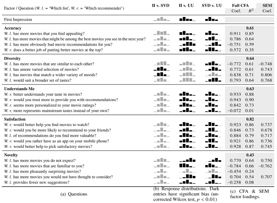
Survey Design
Initial ‘which do you like better?’
22 questions
- ‘Which list has more movies that you find appealing?’
- ‘much more A than B’ to ‘much more B than A’
- Target 5 concepts
Final ‘which do you like better?’
Example Questions
- Diversity
Which list has a more varied selection of movies?
- Satisfaction
Which recommender would better help you find movies to watch?
- Novelty
Which list has more movies you do not expect?
Analysis features
- joint evaluation
- users compare 2 lists
- judgment-making different from separate eval
- enables more subtle distinctions
hard to interpret
- factor analysis
- 22 questions measure 5 factors
- more robust than single questions
structural equation model tests relationships
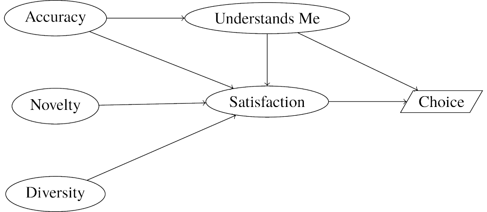
Hypothesized Model
Response Summary
582 users completed
| Condition (A v. B) | N | Pick A | Pick B | % Pick B |
|---|---|---|---|---|
| I-I v. U-U | 201 | 144 | 57 | 28.4% |
| I-I v. SVD | 198 | 101 | 97 | 49.0% |
| SVD v. U-U | 183 | 136 | 47 | 25.7% |
bold is significant (\(p < 0.001\), \(H_0: b/n = 0.5\))
Question Responses
Measurement Model
- Multi-level linear model
- Direction comes from theory
- Condition variables omitted for simplicity
Differences from Hypothesis
- No Accuracy, Understands Me
- Edge from Novelty to Diversity
RQ1: Factors of Choice
Choice: Satisfaction
Satisfaction positively affects impression and choice.
Choice: Diversity
Diversity positively influences satisfaction.
- Satisfaction mediates diversity's impact on preference
Choice: Novelty
Novelty hurts satisfaction and choice/preference.
Choice: Novelty (cont.)
Novelty improves diversity (slightly).
- outweighed by negative satisfaction effect
Choice: Novelty (cont.)
Novelty has direct negative impact on first impression.
- Also seems stronger overall, but difficult to assess
Implications
Novelty boosts diversity, but hurts algorithm impression
- In context of choosing an algorithm
Negative impact of novelty diminishes with close scrutiny
- Can recommender get less conservative as users gain experience?
Diversity has positive impact on user satisfaction
Diversity does not trade off with perceived accuracy
RQ2: Algorithm Differences
- Pairwise comparisons very difficult to interpret
Method: re-interpret as 3 pseudo-experiments
- Use one algorithm as baseline
- User evaluates 1 other, with reference to baseline
- E.g.: judge I-I or U-U, comparing to SVD
- Randomization lets this work (mostly)
Re-use SEM — now condition indicator variable works
Measurement Model
RQ2: Algorithm Differences
- User-user more novel than either SVD or item-item
- User-user more diverse than SVD
- Item-item slightly more diverse than SVD (but diversity didn't affect satisfaction)
- User-user's excessive novelty decreases for experienced (many ratings) users
- Users choose SVD and item-item in roughly equal measure
- Results consistent with raw responses
Choice in Pseudo-Experiments
| Baseline | Tested | % Tested > Baseline |
|---|---|---|
| Item-Item | SVD | 48.99 |
| User-User | 28.36 | |
| SVD | Item-Item | 51.01 |
| User-User | 25.68 | |
| User-User | Item-Item | 71.64 |
| SVD | 74.32 |
RQ3: Objective Properties
Measure objective features of lists:
- Novelty
obscurity (popularity rank)
- Diversity
intra-list similarity (Ziegler)
- Sim. metric: cosine over tag genome (Vig)
- Also tried rating vectors, latent feature vectors
- Accuracy/Sat
RMSE over last 5 ratings
Relativize: take log ratio of two lists' values
Property Distributions
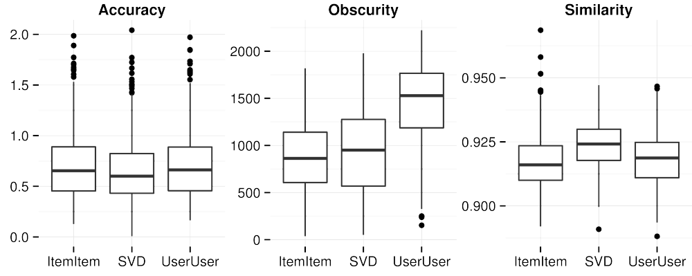
- Obscurity & similarity metrics consistent with RQ2 results
Model with Objectives
- Each metric predicts feature
- Metric effect entirely mediated
Summary
Novelty has complex, largely negative effect
- Exact use case likely matters
- Complements McNee's notion of trust-building
Diversity is important, mildly influenced by novelty.
- Tag genome measures perceptible diversity best, but advantage is small.
User-user loses (likely due to obscure recommendations), but users are split on item-item vs. SVD
Consistent responses, reanalysis, and objective metrics
Results and Expectations
Commonly-held offline beliefs:
- Novelty is good
- Diversity and accuracy trade off
Perceptual results (here and elsewhere):
- Novelty is complex
- Diversity and accuracy both achievable
Remaining Questions
- Are II/SVD interchangeable?
- Can user-user be fixed w/ hybridization?
Do users' stated choices predict long-term preference?
- Will test when ML deploys pick-your-algorithm feature
Overview
Contributions
To promote recommender engineering:
LensKit toolkit for reproducible recommender research
New advances in configuring and tuning collaborative filtering algorithms
Demonstrated differences between algorithms in terms of correct predictions
Demonstrated user-perceptible differences between recommender algorithms, and factors important to user choice
Future Work
Follow up on online experiment
- Long-term user behavior
- Integrate with Kluver's results
LensKit enhancements
- Better new user experience (docs, examples)
- Implicit feedback support
- Temporal evaluation
- Automatic tuning
Much more work needed for engineering
Thank you!
Also thanks to
- Excellent collaborators
- Jennifer for supporting me
- GroupLens Research for amazing support
- NSF for funding research
The Noun Project for great icons
- ‘Document’ by Rob Gill
- ‘Test Tube’ by Olivier Guin
- ‘Experiment’ by Icons Pusher
- ‘Future’ by Megan Sheehan
Correlation Functions
Difference is in summing domains.
- Pearson: items rated by both
- Cosine: union of items, missing ratings 0 offset
